The Map, Shuffle, and Reduce Pattern

"I spent the whole job sitting on a key, waiting for my values to arrive from across the cluster. The map workers were done in seconds. I waited for the network all afternoon."

A Reducer That Has Seen the Shuffle

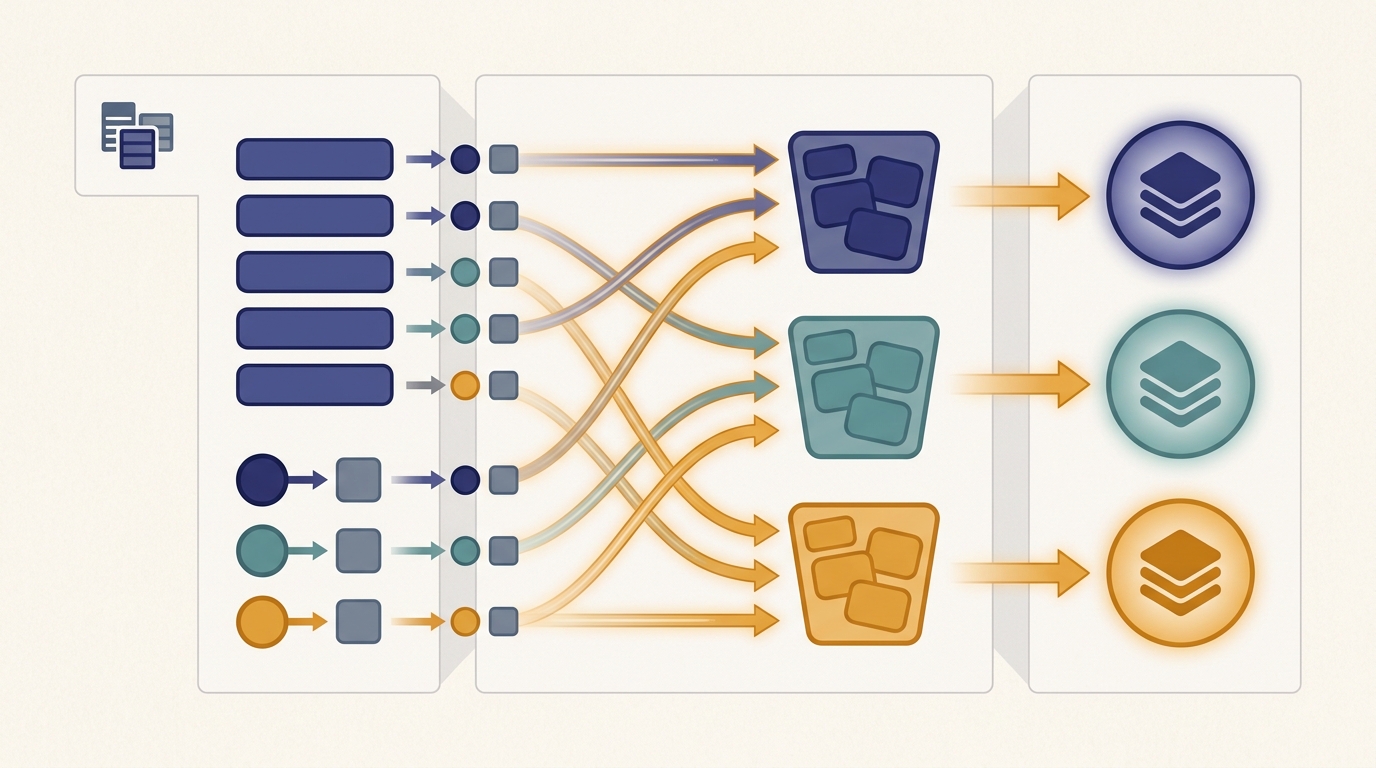
Section 6.1 motivated MapReduce as the answer to a recurring problem: a computation whose input is too large for one machine but whose structure is "do the same independent thing to every record, then combine." This section opens that structure up. A MapReduce job is three phases that always run in the same order. The map phase applies a function to each input record and emits intermediate key-value pairs. The shuffle phase, supplied entirely by the framework, groups every emitted value by its key and moves it across the network to the worker that will reduce that key. The reduce phase applies a function to all the values for a single key and emits the final output. The programmer writes the map and the reduce; the framework owns the shuffle, the parallelism, the partitioning, and the fault tolerance. Holding that division of labor in mind is the whole game, so we draw it before we dissect it.

1. Map: One Function, Every Record, In Parallel Beginner

The map phase is the easy half of MapReduce, and its ease is the whole point. The framework slices the input into fixed-size pieces called input splits, typically the blocks of a distributed filesystem, and assigns one map task per split. Each map task reads its split record by record and calls your map function on each record. The map function returns zero or more intermediate key-value pairs. Counting words, the map receives a line and emits one $(\text{word}, 1)$ pair per word; building an inverted index, it receives a document and emits one $(\text{term}, \text{docID})$ pair per term. The crucial property is that map tasks are completely independent: no map task reads another's input, sees another's output, or waits on another. This is the embarrassingly parallel structure from Section 6.1, and it means the map phase scales linearly with the number of workers up to the number of splits.

Because the work is per record and stateless across records, the framework is free to place each map task on the machine that already holds its split, so the input never crosses the network. That choice is not an accident; it is the data-locality principle from Section 2.8, applied at the granularity of a filesystem block. Moving computation to data is cheap; moving data to computation is the thing we are trying to avoid. The map phase honors that rule perfectly, which is precisely why all the unavoidable data movement gets pushed into the next phase.

2. Shuffle: The Phase That Costs Intermediate

Between map and reduce sits the shuffle, the only phase the programmer never writes and the only phase that is communication rather than computation. Its job is a global group-by: every intermediate pair emitted by every map task must be delivered to the single reduce task responsible for its key. The framework decides which reducer owns which key with a partition function, almost always $\text{partition}(k) = \operatorname{hash}(k) \bmod R$ for $R$ reduce tasks, so that the same key from every map task lands on the same reducer. Each map task therefore writes its output into $R$ buckets, sorted by key; each reduce task then pulls its bucket from all $M$ map tasks, producing $M \times R$ transfers across the network.

This all-to-all movement is why the shuffle dominates. The map phase touched data already local to each worker; the reduce phase will touch data already gathered on each reducer; but the shuffle, sitting between them, must physically relocate essentially the entire intermediate dataset across the cluster fabric. Its cost scales with the volume of intermediate data, not the cleverness of your map function, and it is bounded by network bandwidth, not by how fast the CPUs compute. If we let $V$ be the total bytes emitted by the maps and $B$ the effective bisection bandwidth of the cluster, the shuffle cannot finish faster than roughly $V / B$, no matter how many cores you add. Adding map and reduce workers speeds the cheap phases and leaves this floor untouched, which is the MapReduce face of the communication-versus-computation tension that Chapter 3 models with the alpha-beta cost law.

3. Reduce: Combine All Values for a Key Beginner

Once the shuffle has gathered every value for a key onto its reducer, the reduce phase is again cheap and local. Each reduce task iterates over its assigned keys; for each key it receives the key and an iterator over all the values that were emitted for it anywhere in the cluster, and it calls your reduce function to fold those values into a final result. Word count sums the ones to a total; an inverted index concatenates the document IDs into a posting list; an average sums the values and divides by the count. Like the map, the reduce is a pure function with no awareness that its inputs traveled across the network to reach it, and reduce tasks are independent of one another, so the reduce phase parallelizes across the $R$ reducers exactly as the map parallelized across the $M$ mappers.

There is a subtlety worth stating plainly, because it sets up the combiner. The reduce function for many useful jobs is associative and commutative: the order in which you fold the values does not change the answer, and you may fold subsets first and combine the subtotals later. Summation, counting, maximum, minimum, and set union all have this property; computing a median or an exact distinct count does not. When the reduce is associative and commutative, the framework is free to do part of the reducing early, before the shuffle, while the data is still local to each map task. That early, map-side reduction is the combiner, and it is the cheapest large win in all of MapReduce.

4. Combiners: Pre-Aggregate to Shrink the Shuffle Intermediate

A combiner is a reduce that runs on the map side, on one map task's output, before anything is shuffled. If a map task counting words emits $(\texttt{the}, 1)$ ten thousand times within its split, shuffling ten thousand identical pairs to a reducer that will only add them up is pure waste. A combiner collapses those ten thousand pairs into a single $(\texttt{the}, 10000)$ pair locally, and only that one pair crosses the network. Because the reduce is associative and commutative, the reducer reaches the identical final answer whether it sums ten thousand ones or one ten-thousand: the combiner changes the shuffle volume, never the result. In the language of Chapter 4, the combiner is a local reduction performed before the collective, the same trick that reduce-scatter uses to avoid moving redundant data.

The demonstration below builds all four stages, map, combine, shuffle, and reduce, as separate Python functions over a synthetic log dataset, and measures the shuffle in bytes with the combiner off and on. The reduce computes per-status total bytes and request counts, an associative-commutative aggregation, so the combiner is safe. We assert that the final result is byte-for-byte identical in both runs and report how much the combiner shrank the data that would cross the network.

import random
from collections import defaultdict

# ---- A small dataset: simulated server log lines "<status> <bytes>" ----
random.seed(7)
statuses = ["200", "200", "200", "404", "500", "301"]   # skewed toward 200
records = [f"{random.choice(statuses)} {random.randint(50, 5000)}"
           for _ in range(20_000)]

K = 4
splits = [records[i::K] for i in range(K)]              # 4 input splits, one per map task

def emit_size(value):
    """Cost model for one shuffled key-value pair, in bytes (key + 8-byte int)."""
    return len(value[0]) + 8

# ---- MAP: each split -> list of (status, bytes) pairs, fully independent ----
def map_phase(split):
    out = []
    for line in split:
        status, nbytes = line.split()
        out.append((status, int(nbytes)))             # emit key-value pair
    return out

mapped = [map_phase(s) for s in splits]                # runs in parallel, per split

# ---- COMBINE: map-side pre-aggregation (sum + count) per split ----
def combine_phase(pairs):
    agg = defaultdict(lambda: [0, 0])                  # key -> [sum, count]
    for k, v in pairs:
        agg[k][0] += v
        agg[k][1] += 1
    return [(k, tuple(sv)) for k, sv in agg.items()]

combined = [combine_phase(p) for p in mapped]

# ---- SHUFFLE: group all emitted values by key across every map task ----
def shuffle_phase(per_split_pairs):
    grouped = defaultdict(list)
    bytes_moved = 0
    for pairs in per_split_pairs:
        for k, v in pairs:
            grouped[k].append(v)
            bytes_moved += emit_size((k, v))
    return grouped, bytes_moved

shuf_raw,  bytes_no_combiner   = shuffle_phase(mapped)
shuf_comb, bytes_with_combiner = shuffle_phase(combined)

# ---- REDUCE: combine all values for a key into the final answer ----
def reduce_raw(values):       return (sum(values), len(values))            # list of ints
def reduce_combined(values):  return (sum(v[0] for v in values),
                                      sum(v[1] for v in values))           # list of (sum,count)

final_no_combiner   = {k: reduce_raw(v)      for k, v in shuf_raw.items()}
final_with_combiner = {k: reduce_combined(v) for k, v in shuf_comb.items()}

print("status   total_bytes        count   mean_bytes")
for k in sorted(final_no_combiner):
    s, c = final_no_combiner[k]
    print(f"{k:>6}   {s:>12,}   {c:>7,}   {s / c:>9.1f}")

assert final_no_combiner == final_with_combiner, "combiner must not change the result"
print()
print(f"distinct keys (reducers)        : {len(shuf_raw)}")
print(f"pairs shuffled, no combiner     : {sum(len(v) for v in shuf_raw.values()):,}")
print(f"pairs shuffled, with combiner   : {sum(len(v) for v in shuf_comb.values()):,}")
print(f"shuffle bytes, no combiner      : {bytes_no_combiner:,}")
print(f"shuffle bytes, with combiner    : {bytes_with_combiner:,}")
print(f"shuffle volume reduction        : "
      f"{100 * (1 - bytes_with_combiner / bytes_no_combiner):.1f}%")
print(f"identical final result?         : {final_no_combiner == final_with_combiner}")

status   total_bytes        count   mean_bytes
   200     25,423,448    10,008      2540.3
   301      8,226,535     3,306      2488.4
   404      8,421,284     3,322      2535.0
   500      8,473,105     3,364      2518.8

distinct keys (reducers)        : 4
pairs shuffled, no combiner     : 20,000
pairs shuffled, with combiner   : 16
shuffle bytes, no combiner      : 220,000
shuffle bytes, with combiner    : 176
shuffle volume reduction        : 99.9%
identical final result?         : True

The 99.9% figure is dramatic because the key space here is tiny, only four distinct status codes, so each split's twenty thousand pairs fold into four. The combiner's payoff is exactly proportional to how many records share a key within a single split: high for low-cardinality aggregations like counts and sums, modest when keys are nearly unique, and zero when every key appears once. A combiner is only legal when the reduce is associative and commutative, and the framework may call it zero, one, or many times, so it must never change the result, only its volume. Output 6.2.1 confirms both halves of that contract: large volume reduction, identical answer.

5. Why This Pattern Generalizes Intermediate

The map-shuffle-reduce shape is narrow on purpose, and its narrowness is its strength. Any computation you can phrase as "transform each record independently, then group by some key and combine each group" fits the pattern, and an astonishing range of data work has that shape: counting, summing, averaging, filtering, building indexes, deduplicating, joining two datasets on a key, and the distributed sorts and graph algorithms that fill the rest of this chapter. The next section, Section 6.3, works the canonical examples, word count and inverted indexing, end to end and shows the combiner cutting their shuffle just as it did here. Because every such job decomposes into the same three phases, the framework can provide partitioning, parallel scheduling, shuffle, and fault tolerance once and reuse them for all of them; the programmer only ever changes the two pure functions at the ends.

Fault tolerance deserves a closing word, because it follows directly from the purity of the two functions. Since a map task is a deterministic function of its split and depends on nothing else, the framework can re-run a failed or straggling map task on another machine and get the same output; the same holds for a reduce task given its shuffled input. That is MapReduce's whole fault-tolerance story, re-execute the failed deterministic piece, and it works only because no task shares mutable state with another. The mechanism and its limits, including what happens when a reducer's input is lost and the shuffle must be partly replayed, are the subject of Section 6.9; for now, note that the same property that made the phases parallel, statelessness, is what makes them recoverable.

from pyspark import SparkContext
sc = SparkContext.getOrCreate()

logs = sc.textFile("hdfs:///logs/*")               # input splits -> map tasks, placed near data
pairs = logs.map(lambda line: (line.split()[0],    # MAP: emit (status, (bytes, 1))
                               (int(line.split()[1]), 1)))
totals = pairs.reduceByKey(lambda a, b:            # COMBINE on the map side, then SHUFFLE,
                           (a[0] + b[0], a[1] + b[1]))   # then REDUCE, all in one call
print(totals.collect())                            # [('200', (25423448, 10008)), ...]

6. The Shuffle as a Research Frontier Advanced

The lesson that the shuffle dominates has not aged; it has migrated. Modern data and AI systems still spend much of their wall-clock moving intermediate data by key, and two decades after MapReduce named the problem, the shuffle is still where the active engineering happens.

With the three phases dissected and the combiner in hand, we can now write real algorithms in this model. The next section turns map, shuffle, and reduce into working key-value computations, word count and the inverted index that powers every search engine, and shows the same combiner that shrank our log shuffle shrinking theirs. That tour begins in Section 6.3.