Push-Pull Architecture

"I hold every parameter and remember every step the optimizer ever took. The workers? They borrow a few rows, hand me a gradient, and forget everything. We get along."

A Parameter Server Under Mild Staleness

Section 11.1 argued why a parameter server exists at all: when a model is dominated by a giant sparse table, such as the embedding rows of a recommendation system, replicating the whole model on every worker (the all-reduce assumption of data-parallel training) is wasteful, because any single batch touches only a vanishing fraction of the rows. The remedy is to keep one authoritative copy of the parameters on a server and let workers borrow slices of it. Now we make that concrete. What exactly does a worker send and receive, in what order, and who holds the optimizer state? The answers define the push-pull architecture, and they are simpler than the machinery they replace.

1. The Pull-Compute-Push Cycle Beginner

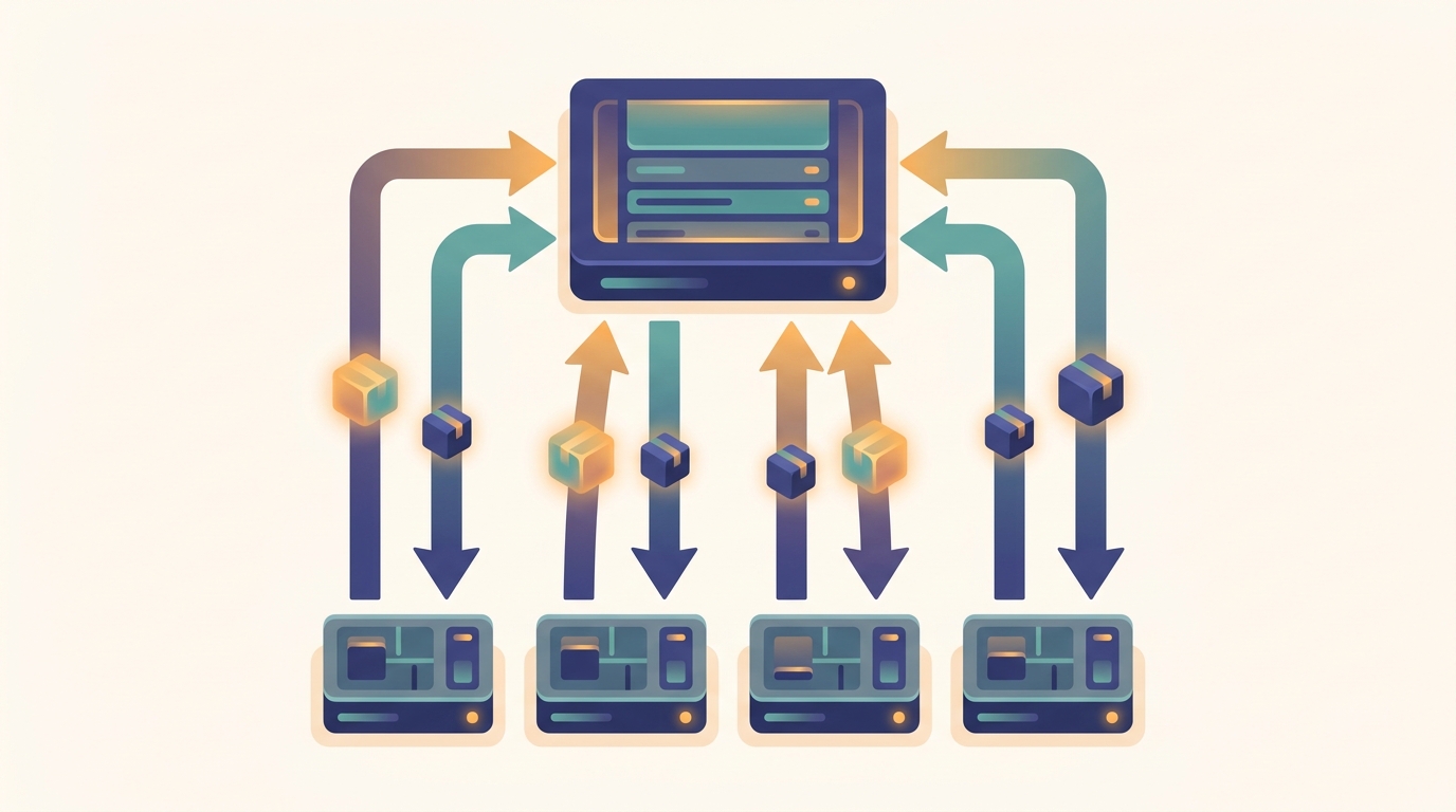
One training iteration on a parameter server is three steps, always in the same order. First the worker pulls: it asks the server for the current value of the parameters it is about to use and receives a copy. Second it computes: using its local batch and the pulled parameters, it runs a forward and backward pass and produces a gradient, a vector the same shape as the parameters it pulled. Third it pushes: it sends that gradient to the server, which applies the update to its authoritative copy. The worker keeps nothing between iterations; on the next step it pulls fresh values again. This is the defining asymmetry of the architecture, and it is worth stating plainly.

Contrast this with the data-parallel all-reduce of Chapter 1, where every worker holds a full copy of the model and its own optimizer state, and the workers average their gradients among themselves with no central party. There, the model state is replicated and symmetric; here, it is centralized and the workers are bare compute. The parameter server trades the symmetry of all-reduce for the ability to hold a model far larger than any one worker could, fetched a slice at a time. Figure 11.2.1 shows the cycle and the slice.

2. Range Pulls and Keyed Sparse Pulls Beginner

How much does a worker pull? The naive answer, the whole model, is exactly what we are trying to avoid. The parameter-server API instead lets the worker name what it wants, and two naming schemes cover almost every case. A range pull asks for a contiguous block of parameters, say rows $[1000, 2000)$; it suits dense layers and any parameter laid out as one contiguous array, and it is cheap to express because a range is two integers. A keyed sparse pull asks for an explicit list of keys, say rows $\{7, 42, 88, \dots\}$; it suits embedding tables, where a batch references a scattered, data-dependent handful of rows out of millions or billions. The keyed pull is the workhorse of this chapter, because the sparse embedding table is precisely the model that motivated parameter servers in Section 11.1.

The arithmetic is the whole point. Suppose the table has $V$ rows of width $D$, so the full model is $V \cdot D$ numbers. A batch of $B$ examples, each referencing a few features, touches at most some number $m$ of distinct keys, and typically $m \ll V$. A keyed pull moves $m \cdot D$ numbers down and the matching gradient moves $m \cdot D$ numbers back up, for a round-trip cost of $2 m D$. The ratio of a dense pull to a sparse round trip is therefore roughly $V / (2m)$, which for a million-row table touched by a few hundred keys is a saving of nearly three orders of magnitude. We do not have to take that on faith.

3. Building the Push-Pull API from Scratch Intermediate

The cleanest way to see the architecture is to implement it. The code below is a complete, in-process parameter server in pure Python: a server that owns a keyed table and an Adagrad accumulator, a pull that returns only the requested rows, a push that applies the update server-side, and a stateless worker that strings the three steps together. We then run eight workers, each with a batch that touches a few dozen random keys out of a million-row table, and we count the numbers that actually crossed the wire against the cost of pulling the whole table once.

import random
random.seed(0)

VOCAB, DIM, LR = 1_000_000, 16, 0.05      # table rows, row width, learning rate

class ParameterServer:
    """Owns the table AND the optimizer state; the only party that applies updates."""
    def __init__(self, dim):
        self.table, self.accum, self.dim = {}, {}, dim
        self.pull_numbers = self.push_numbers = 0     # bytes-on-wire counters

    def _row(self, key):                              # lazy init: rows exist on first touch
        if key not in self.table:
            self.table[key] = [0.01 * (i + 1) for i in range(self.dim)]
            self.accum[key] = [1e-8] * self.dim
        return self.table[key]

    def pull(self, keys):                             # keyed sparse pull: ONLY these rows
        rows = {k: list(self._row(k)) for k in keys}
        self.pull_numbers += len(keys) * self.dim
        return rows

    def push(self, grads):                            # server-side Adagrad update
        for k, g in grads.items():
            acc, row = self.accum[k], self.table[k]
            for i in range(self.dim):
                acc[i] += g[i] * g[i]
                row[i] -= LR * g[i] / (acc[i] ** 0.5)
        self.push_numbers += len(grads) * self.dim

def worker_step(server, batch_keys):                  # stateless: pull, compute, push, forget
    rows  = server.pull(batch_keys)                   # 1. pull touched rows
    grads = {k: [v * 0.1 for v in vec] for k, vec in rows.items()}   # 2. toy gradient
    server.push(grads)                                # 3. push gradient back

ps = ParameterServer(DIM)
batches = [[random.randrange(VOCAB) for _ in range(64)] for _ in range(8)]   # 8 workers
touched = set()
for b in batches:
    worker_step(ps, b)
    touched.update(b)

dense = VOCAB * DIM                                   # cost of pulling the whole table once
sparse = ps.pull_numbers + ps.push_numbers
print(f"table rows (vocab)        : {VOCAB:,}")
print(f"dense pull of full table  : {dense:,} numbers")
print(f"distinct keys touched     : {len(touched):,}")
print(f"pull volume (8 workers)   : {ps.pull_numbers:,} numbers")
print(f"push volume (8 workers)   : {ps.push_numbers:,} numbers")
print(f"sparse round-trip total   : {sparse:,} numbers")
print(f"reduction vs dense pull    : {dense / sparse:,.0f}x")
print(f"rows materialized on server: {len(ps.table):,}")

table rows (vocab)        : 1,000,000
dense pull of full table  : 16,000,000 numbers
distinct keys touched     : 511
pull volume (8 workers)   : 8,192 numbers
push volume (8 workers)   : 8,192 numbers
sparse round-trip total   : 16,384 numbers
reduction vs dense pull    : 977x
rows materialized on server: 511

Two details in Code 11.2.1 carry the architecture. The server initializes rows lazily, so a billion-row table costs nothing until a key is actually referenced; only the 511 touched rows were ever materialized. And the optimizer state, the Adagrad accumulator accum, lives entirely on the server and is updated inside push; the worker never sees it, which is what keeps the worker stateless and replaceable. The communication saving is not a trick of this toy: it is the structural reason a parameter server can host a model that no single worker could hold.

import torch
from torchrec import EmbeddingBagConfig, EmbeddingBagCollection, KeyedJaggedTensor

ebc = EmbeddingBagCollection(tables=[
    EmbeddingBagConfig(name="item", embedding_dim=16,
                       num_embeddings=1_000_000, feature_names=["item"])],
    device=torch.device("cpu"))

# A batch that references only a handful of keys out of a million rows.
batch = KeyedJaggedTensor.from_lengths_sync(
    keys=["item"], values=torch.tensor([7, 42, 88]), lengths=torch.tensor([1, 1, 1]))

pooled = ebc(batch)          # sparse pull + lookup; backward() pushes the gradient

4. This Is Broadcast-and-Gather, Not All-Reduce Intermediate

It is worth naming the communication pattern precisely, because the contrast with data-parallel training is the conceptual hinge of this chapter. In all-reduce, every worker contributes a gradient and every worker receives the same averaged result; the operation is symmetric, peer-to-peer, and has no privileged node. The push-pull cycle is not that. A pull is a broadcast from the server outward: the server holds the parameters and sends slices to whichever workers ask. A push is a gather inward: many workers send gradients to the one server that owns the update. The pattern is the broadcast-and-gather pair that Section 4.7 introduced as the movement of weights outward and experience inward, and a parameter server is that pair run on every step.

This is why a parameter server is the natural home for a sparse model and all-reduce is not. All-reduce sums full gradient vectors of identical shape across peers; it has no way to say "I only touched 511 rows, sum just those." The broadcast-and-gather of push-pull is keyed by construction: the worker names its rows on the way out and names them again on the way back, so sparsity is expressed for free. Chapter 10 framed distributed optimization as the general problem of combining gradients computed on partitioned data; the parameter server is the combine-at-a-central-owner answer, in contrast to the combine-among-peers answer of all-reduce that Chapter 6 previewed through the MapReduce shuffle.

5. Cutting Round Trips: Batching and Compression Intermediate

Every pull-compute-push cycle pays at least one network round trip, and on a real cluster the latency of that round trip, not the bytes, is often what limits throughput. Two standard moves attack it. The first is message batching: instead of one pull request per feature, a worker coalesces all the keys its batch touches into a single pull message, and the server returns all the rows in one response; the eight workers in Code 11.2.1 already do this, issuing one keyed pull each rather than 64 separate ones. The second is compression: the rows and gradients on the wire can be sent in lower precision (16-bit or 8-bit instead of 32-bit) or, for the gradient push, quantized and sparsified further, since a sparse model's gradients are themselves often near zero in most coordinates. These reduce the bytes per round trip, complementing the keyed pull that already reduced the number of rows.

There is a deduplication win hiding in the batching too. If two examples in the same batch reference key 42, the worker should pull row 42 once, not twice; coalescing keys into a set before the pull (exactly what the touched set models in Code 11.2.1) removes the duplication before it reaches the wire. Across many workers the same row is often hot, referenced by most batches, which is both an opportunity (cache it) and a hazard (a contention hot spot on the server that owns it), a tension Section 11.3 addresses by sharding the table across many servers so that no single row owner becomes the bottleneck.

6. Consistency When Workers Interleave Advanced

A single worker's pull-compute-push cycle is clean: it pulls the current parameters, computes a gradient on exactly those values, and pushes it back. The subtlety appears the moment a second worker shares the server. Suppose worker A pulls row 42, and before A pushes its gradient, worker B pulls the same row 42, computes, and pushes first. Now A's gradient was computed on a value of row 42 that is already stale, because B's update has landed in between. A's push still applies, but it applies a gradient that does not correspond to the row's current state. The model still moves in a roughly correct direction, yet the clean per-worker identity of pull-compute-push no longer holds across the cluster.

How much this matters, and what to do about it, is the entire subject of the next two sections. One option is to forbid the interleaving: make every worker pull a consistent snapshot and apply updates in a strict order, which is correct but forces workers to wait on each other (synchronous updates). The other is to embrace the interleaving: let workers pull, compute, and push without coordination and accept that gradients are computed on slightly stale parameters (asynchronous updates), trading a little staleness for a lot of throughput. The push-pull API is identical in both regimes; what changes is the consistency the server promises about the values a pull returns. We make that trade precise, and bound the staleness, in Section 11.4.

We now have the API (pull, compute, push), the saving that justifies it (keyed sparse pulls that move bytes proportional to keys touched, as Output 11.2.1 made concrete), and its place in the taxonomy (broadcast-and-gather, not all-reduce). What we have quietly assumed is a single server holding the whole table. That assumption breaks at scale: one server cannot hold a terabyte table or absorb the gather traffic of a thousand workers. Section 11.3 lifts it, sharding the parameters across many servers while keeping the push-pull contract from this section unchanged.