"They built me a room with eight specialists and a receptionist who reads two words of your problem before deciding which two of us you get. I am the specialist nobody's two words ever point to."
An Expert Nobody Routed To
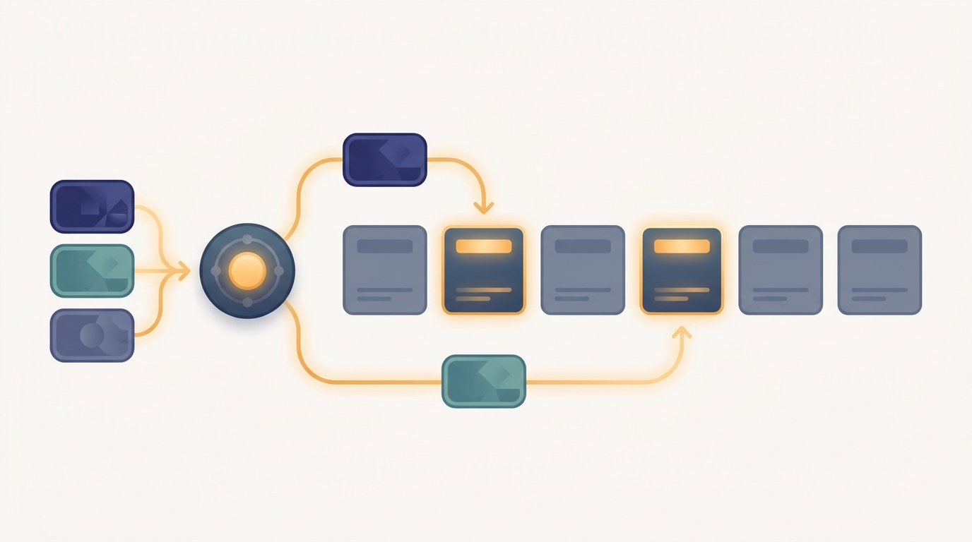
A Mixture-of-Experts layer replaces the single dense feed-forward sublayer of a transformer with many parallel expert feed-forward networks and a small gating network that, for each token, selects only a few experts to run. The layer holds the parameters of all experts but spends compute on only the chosen handful, so the parameter count grows while the work per token stays nearly flat. That decoupling of capacity from cost is the entire reason sparse models exist, and it is what Section 17.1 framed as dense versus sparse scaling. The mental model above captures the whole idea in one image: a router sends each token to only one or two of many experts, so most experts stay idle for any given token. This section dissects that picture into one MoE layer: what an expert is, how the gate picks experts, how the chosen outputs are combined into one vector, and why the feed-forward sublayer is the natural place to do all of this. The selected experts will later live on different machines, which is what turns this local layer into the distributed problem the rest of the chapter solves.
In Chapter 15 every worker held a full copy of the same dense model and the only thing that differed across machines was the data. A Mixture-of-Experts model breaks that symmetry: the model itself contains parts that most tokens never touch. To see how, we zoom all the way in to a single transformer block and change exactly one sublayer. Recall that a transformer block alternates an attention sublayer, which mixes information across positions, with a position-wise feed-forward network (FFN) that transforms each token independently. The FFN is where Mixture-of-Experts does its work, because it is both the heaviest part of the block and the part that already treats every token on its own.
1. From One Feed-Forward Network to Many Experts Beginner
The dense feed-forward sublayer applies the same two-layer network to every token vector $x \in \mathbb{R}^{d}$, expanding to a hidden width $h$ and projecting back: $\mathrm{FFN}(x) = \sigma(x W_1) W_2$, with $W_1 \in \mathbb{R}^{d \times h}$ and $W_2 \in \mathbb{R}^{h \times d}$. Because $h$ is typically four times $d$, this one sublayer holds roughly two thirds of the parameters in a transformer block, and every token pays for all of them on every forward pass. That is the cost a Mixture-of-Experts layer attacks.
The construction is direct. Instead of one FFN, install $E$ separate feed-forward networks, called experts, each with its own weights $W_1^{(e)}, W_2^{(e)}$ and identical shape. Add a small gating network $g$ that reads the token and decides which experts should handle it. The layer's output for a token is then a weighted sum over the experts the gate selected, not over all of them. With $E$ experts the layer stores $E$ times as many feed-forward parameters as a dense block, yet if the gate picks only $k$ of them per token, the compute per token rises by a factor of $k$, not $E$. Choosing $k = 2$ while $E = 64$ buys thirty-two times the feed-forward capacity for twice the feed-forward compute.
A dense layer ties parameters to compute: every parameter is multiplied for every token. An MoE layer cuts that tie. Total capacity scales with the number of experts $E$, but compute per token scales with the number selected $k$, and $k$ is held small and fixed (usually 1 or 2). You add knowledge to the model by adding experts, which costs memory and, once experts span machines, communication, but you do not add floating-point work per token. Every distributed challenge in this chapter (sharding experts, routing tokens, balancing load) is the price of keeping that decoupling intact at scale.
2. The Gate: Scoring and Top-k Selection Intermediate
The gating network is deliberately tiny, usually a single linear layer. For a token $x$ it produces one score per expert, $s = x W_g$ with $W_g \in \mathbb{R}^{d \times E}$, giving a vector of $E$ logits. The gate then keeps the $k$ largest of those logits, the token's top-$k$ experts, and discards the rest. Crucially, the softmax that turns scores into combination weights is taken over only the selected experts, not all $E$, so the weights of the chosen experts sum to one and the unchosen experts contribute nothing. Writing $\mathcal{T}(x)$ for the set of top-$k$ expert indices, the gate weight for a selected expert $e$ is
$$ G_e(x) = \frac{\exp\!\big(s_e\big)}{\sum_{j \in \mathcal{T}(x)} \exp\!\big(s_j\big)}, \qquad e \in \mathcal{T}(x), $$and $G_e(x) = 0$ for every expert outside $\mathcal{T}(x)$. The layer output is the gate-weighted combination of the selected experts' feed-forward outputs,
$$ y = \sum_{e \in \mathcal{T}(x)} G_e(x)\, \mathrm{FFN}_e(x) = \sum_{e \in \mathcal{T}(x)} G_e(x)\, \sigma\!\big(x W_1^{(e)}\big) W_2^{(e)}. $$This is the gated combination at the heart of the layer, and it is worth reading carefully. The sum runs over only $k$ experts, so only $k$ feed-forward networks are ever evaluated for this token. The weights $G_e(x)$ are produced by the gate from the same token, so the routing is learned end to end: the gradient flows back through $G_e(x)$ into $W_g$, teaching the gate which experts serve which tokens. We treat the design of that learning signal, including how to stop the gate from collapsing onto a few favorite experts, as its own subject in Section 17.3. Here the gate is just the mechanism that selects and weights.
3. Why the Feed-Forward Sublayer Is the Place to Sparsify Intermediate
One might ask why the experts replace the feed-forward sublayer rather than the attention sublayer. Three properties of the FFN make it the natural target. First, it carries the parameters: with hidden width $h \approx 4d$, the two feed-forward matrices dominate the block's weight count, so multiplying that sublayer by $E$ is where extra capacity actually lands. Second, it is already position-wise. The FFN transforms each token independently of the others, so routing each token to its own experts changes nothing about the layer's structure; attention, by contrast, mixes tokens together, and splitting it per token would break the very communication it exists to provide. Third, the routing decision is cheap relative to the FFN it gates. A single linear gate over $E$ experts costs $d \cdot E$ multiplies per token, negligible beside the $\mathcal{O}(d h)$ of even one expert, so selection adds almost nothing to the bill it controls.
The result is a layer that is a drop-in replacement: the surrounding attention, residual connections, and normalization are untouched, and only the FFN becomes a routed set of FFNs. A common pattern places an MoE layer in every other transformer block, leaving the rest dense, so a model is sparse where capacity pays off and dense where it does not. This is the same partition-the-heavy-part instinct that drove sharding in Chapter 16; there we split one big matrix across devices, here we split capacity across many specialized matrices and route to a few.
Picture a clinic. The dense FFN is one exhausted generalist who sees every patient and must know everything. The MoE layer hires a panel of specialists and a fast receptionist who reads the first line of each complaint and waves the patient toward the two most relevant doctors. The clinic now holds far more expertise, yet each patient still sees only two people, so no visit takes longer. The receptionist is the gate, and the whole trick is that the panel can grow without lengthening anyone's appointment.
4. Shared and Routed Experts Intermediate
Pure top-$k$ routing has a subtle inefficiency: knowledge that every token needs, basic grammar, common formatting, must be relearned and duplicated inside many experts, because no single expert is guaranteed to be on the route for any given token. Several recent designs fix this by splitting the experts into two kinds. A small number of shared experts are always active, run for every token regardless of the gate, and absorb the common knowledge. The remaining routed experts are selected top-$k$ as before and specialize. The layer output adds the shared contribution to the routed combination,
$$ y = \sum_{e \in \mathcal{S}} \mathrm{FFN}_e(x) \;+\; \sum_{e \in \mathcal{T}(x)} G_e(x)\, \mathrm{FFN}_e(x), $$where $\mathcal{S}$ is the fixed set of shared experts and $\mathcal{T}(x)$ the token's routed top-$k$. The DeepSeek family popularized this shared-plus-routed structure, isolating common patterns in the always-on experts so the routed experts are free to specialize harder. The cost is modest, one or two extra FFN evaluations per token for the shared experts, and in exchange the routed experts stop wasting capacity on redundancy. We will see in Section 17.3 that this also stabilizes the gate, since the shared path keeps gradients flowing even to tokens whose routing is briefly poor.
5. The Forward Pass, Token by Token Intermediate
It is worth tracing the whole forward pass once at the level of a single token, because every later complication is a distributed version of these four steps. A token vector arrives. The gate scores all $E$ experts and selects the top $k$ (gate). Those $k$ expert FFNs are evaluated on the token, and no others (select and dispatch). Their outputs are scaled by the gate weights and summed (combine). The result replaces what the dense FFN would have produced, and the block continues as usual. The code below builds exactly this on a small batch with pure NumPy, four experts and top-2 routing, so the routing and the combine are fully visible rather than hidden behind a framework.
import numpy as np

rng = np.random.default_rng(7)
T, d, h, E, k = 6, 8, 16, 4, 2        # tokens, model dim, hidden dim, experts, top-k

# One small FFN expert: x -> relu(x W1) W2, each expert has its OWN weights.
W1 = rng.standard_normal((E, d, h)) * 0.3   # per-expert first layer
W2 = rng.standard_normal((E, h, d)) * 0.3   # per-expert second layer

def expert_forward(e, x):                    # FFN of expert e on row-batch x
    return np.maximum(x @ W1[e], 0.0) @ W2[e]

# The gate: a single linear scorer shared by all tokens, one logit per expert.
Wg = rng.standard_normal((d, E)) * 0.5
X = rng.standard_normal((T, d))              # a batch of T token vectors

logits = X @ Wg                              # (T, E) raw expert scores per token
# Top-k selection: keep the k highest logits per token, softmax over JUST those.
topk_idx = np.argsort(-logits, axis=1)[:, :k]          # (T, k) chosen expert ids
topk_logits = np.take_along_axis(logits, topk_idx, 1)  # (T, k) their scores
g = np.exp(topk_logits - topk_logits.max(1, keepdims=True))
gate_w = g / g.sum(1, keepdims=True)                   # (T, k) softmax gate weights

# Forward pass: each token is dispatched ONLY to its k experts, then combined.
Y = np.zeros((T, d))
for t in range(T):
    for j in range(k):
        e = topk_idx[t, j]
        Y[t] += gate_w[t, j] * expert_forward(e, X[t:t+1])[0]

# A dense baseline would run ALL E experts for every token. Count the saving.
sparse_calls = T * k
dense_calls = T * E

print("tokens T, experts E, top-k :", T, E, k)
print("expert-FFN evals (sparse)  :", sparse_calls)
print("expert-FFN evals (dense)   :", dense_calls,
      f"  -> {sparse_calls/dense_calls:.0%} of dense work")
print()
print("per-token routing (expert: gate-weight):")
for t in range(T):
    parts = ", ".join(f"E{topk_idx[t,j]}:{gate_w[t,j]:.2f}" for j in range(k))
    print(f"  token {t}  ->  {parts}")
print()
print("output norms per token     :", np.round(np.linalg.norm(Y, axis=1), 3))
tokens T, experts E, top-k : 6 4 2
expert-FFN evals (sparse)  : 12
expert-FFN evals (dense)   : 24   -> 50% of dense work

per-token routing (expert: gate-weight):
  token 0  ->  E2:0.70, E1:0.30
  token 1  ->  E1:0.85, E3:0.15
  token 2  ->  E3:0.76, E2:0.24
  token 3  ->  E3:0.79, E1:0.21
  token 4  ->  E3:0.93, E0:0.07
  token 5  ->  E2:0.54, E0:0.46

output norms per token     : [1.197 1.095 2.692 1.186 1.313 2.454]
The output makes the layer's character concrete. Token 0 leans on expert 2 with weight 0.70 and expert 1 with 0.30; token 4 sends almost all of its weight, 0.93, to expert 3. No token runs all four experts, the evaluation count is exactly $T \times k = 12$ rather than $T \times E = 24$, and each token's output is a convex combination of just its two specialists. Notice already a hint of the load problem this chapter must solve: expert 3 appears on four of the six tokens while some experts appear rarely, an imbalance that becomes a real cost once experts sit on separate machines and a popular expert's machine is swamped. That is the thread Section 17.6 picks up with load-balancing losses.
Chapter 15 distributed one computation across machines that all held the same model. Mixture-of-Experts distributes the model itself: the experts are different parameters, and at scale they live on different machines, so a token's forward pass becomes a journey across the cluster to reach its chosen experts and back. The combine step you just wrote as a local weighted sum becomes a network operation. In Chapter 15 the binding collective was all-reduce over identical gradients; for routed experts the binding collective is all-to-all, because each machine must hand every other machine the tokens destined for the experts it hosts. The gate in Code 17.2.1 is, quietly, a router that decides who talks to whom, and that is the bridge from this local layer to the distributed system of Sections 17.4 and 17.5.
The hand-written gate, top-$k$ selection, and combine loop in Code 17.2.1 are the parts a production library implements once and tunes hard. In a framework such as PyTorch the same routed layer is a few lines, and the dispatch is vectorized rather than looped:
import torch, torch.nn as nn, torch.nn.functional as F

class MoE(nn.Module):
    def __init__(self, d, h, E, k):
        super().__init__()
        self.k = k
        self.gate = nn.Linear(d, E, bias=False)                 # the router
        self.experts = nn.ModuleList(                           # E independent FFNs
            nn.Sequential(nn.Linear(d, h), nn.ReLU(), nn.Linear(h, d))
            for _ in range(E))

    def forward(self, x):                                       # x: (tokens, d)
        w, idx = self.gate(x).topk(self.k, dim=-1)              # top-k scores + ids
        w = F.softmax(w, dim=-1)                                # gate weights over k
        y = torch.zeros_like(x)
        for j in range(self.k):                                 # one slot at a time
            for e in range(len(self.experts)):
                m = idx[:, j] == e                              # tokens routed to e
                if m.any():
                    y[m] += w[m, j:j+1] * self.experts[e](x[m])
        return y
transformers) replace this per-expert loop with a single batched-dispatch kernel and add the expert sharding and all-to-all that Chapter 16's machinery and Section 17.5 develop, collapsing hundreds of lines of routing, capacity, and communication code into a configured module.Who: A model engineer on a small team training a domain-specific code-and-prose assistant.
Situation: A dense 7-billion-parameter model trained within budget but plateaued in quality; the obvious fix, a 20-billion-parameter dense model, tripled the training and serving FLOPs and blew past the team's GPU-hour allowance.
Problem: They needed substantially more model capacity to absorb a large, diverse corpus, but the compute bill scaled with parameters in a dense model and they could not afford it.
Dilemma: Stay dense and accept the quality ceiling at 7B, or grow dense to 20B and accept the compute they could not pay for. Neither fit.
Decision: They converted the feed-forward sublayers in alternate blocks to MoE layers with $E = 16$ experts and top-$k = 2$ routing, plus one always-on shared expert, raising total parameters near 20B while keeping active parameters per token close to the original 7B.
How: They swapped each chosen FFN for the framework's MoE module (Code 17.2.2's production cousin), kept the gate small and linear, and added the load-balancing loss of Section 17.6 so no expert was starved or swamped.
Result: Quality matched a dense model far larger than 7B while the per-token compute, and therefore the training and inference cost, stayed close to the 7B baseline; the extra parameters lived as memory and routing traffic, not as FLOPs.
Lesson: When capacity is the ceiling and compute is the budget, sparsity buys what dense scaling cannot. The expense moves from arithmetic to memory and communication, which is precisely the bill the rest of this chapter teaches you to manage.
6. What the Layer Sets Up for the Rest of the Chapter Beginner
We now have the anatomy: an MoE layer is $E$ expert FFNs, a linear gate, top-$k$ selection, and a gate-weighted combine, optionally with a few always-on shared experts. Two questions follow immediately, and each owns a later section. First, how should the gate learn to route, and how do we keep it from sending nearly every token to the same few experts? That is routing and gating, the subject of Section 17.3. Second, what happens when the experts are too numerous to fit on one machine and must be spread across the cluster? Then a token's trip to its experts crosses the network, the combine becomes a collective, and load imbalance becomes a hot-machine problem. That is expert parallelism, developed in Sections 17.4 and 17.5, where the all-to-all foreshadowed above becomes the engine of token routing. The local layer in this section is the unit that those sections replicate, shard, and connect.
Mixture-of-Experts moved from research curiosity to the default for frontier-scale open models in this period. Mixtral 8x7B (Jiang et al., 2024) made the top-2-of-8 routed FFN a widely studied baseline, with roughly 47B total parameters but only about 13B active per token. The DeepSeek-V2 and DeepSeek-V3 line (2024 to 2025) pushed fine-grained experts and the shared-plus-routed structure of Section 4, training models with hundreds of billions of total parameters while keeping active parameters small, and reported that isolating common knowledge in shared experts measurably improves the specialization of the routed ones. Qwen and other families shipped MoE variants over the same window. A parallel research thread asks where the gains really come from: studies of expert specialization, of how many experts a token truly needs, and of routing stability question whether top-$k$ is optimal and propose alternatives such as expert-choice routing, which we meet in Section 17.3. The open question driving the field is how far total capacity can outrun active compute before routing quality, not arithmetic, becomes the limit.
Consider a transformer block whose dense FFN has model dimension $d = 4096$ and hidden width $h = 16384$. (a) How many parameters are in the two feed-forward matrices $W_1$ and $W_2$ of this dense FFN? (b) Replace it with an MoE layer of $E = 64$ experts, each the same shape, and top-$k = 2$ routing. How many feed-forward parameters does the layer now hold, and by what factor did capacity grow? (c) Ignoring the gate, by what factor did the feed-forward FLOPs per token grow relative to the dense FFN? (d) Explain in one sentence why the answers to (b) and (c) differ, and connect that gap to the Key Insight of Section 1.
Starting from Code 17.2.1, designate expert 0 as an always-on shared expert: it runs for every token in addition to the routed top-$k$, and its output is added to the routed combination as in the equation of Section 4 (you may give it gate weight 1 rather than a softmax weight). Keep top-$k = 2$ routing over the remaining experts. Re-run the batch and report, for each token, which experts it used and the new output norms. Then count expert-FFN evaluations and compare against both the pure-sparse count from Output 17.2.1 and the dense count. Comment on how much extra compute the shared expert costs and what it buys.
Extend Code 17.2.1 to draw a larger batch, say $T = 2000$ tokens, and tally how many tokens each of the $E$ experts received across the top-$k$ routes. Report the counts, the maximum-to-mean ratio, and the fraction of total load carried by the single busiest expert. Now imagine each expert lives on its own machine. Argue from your numbers how this imbalance would translate into idle and overloaded machines, and estimate how much faster the layer could run if the load were perfectly even. This is the quantity the load-balancing loss of Section 17.6 and the capacity factors of Section 17.7 exist to control.